I understand that we want to replace the indicator function by a smooth function however could you please give more details about the use of l(y.g(x_hat)) ? I don't understand how this loss is affected respectively by y and g(x_hat) and I think it would be clearer with an example.
Thank you for your question and that is true we have been a bit quick during the lecture yesterday.
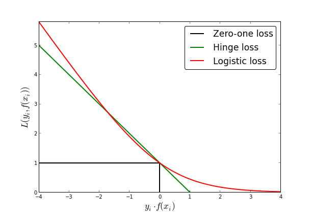
Let's consider a margin-based (i.e., dependent on \(y g(\hat{x})\)) loss function \(\ell(y g(\hat{x})\) such as the logistic loss \( \log(1+e^{-y g(\hat{x}}) \).
(source https://xiucheng.org/2017/01/01/opt4ml.html)
You note that the loss is decreasing.
If you are predicting y by \(g(\hat x)\) then you will pay the price \(\ell(y.g(\hat x))\):
if you are correct, and y and \(g( \hat x)\) are of the same sign, then \( y.g(\hat x)\geq 0\) and the loss value will be small (in fact smaller than the value \(\ell(0)\).
if you are wrong and y and g(x) are of opposite sign, then \( y.g(\hat x)\leq 0\) and the loss value will be large, in fact larger than the value \(\ell(0)\).
So you see that if your loss value \(\ell(y.g(\hat x))\) is larger than \(\ell(0)\), it means than \( y.g(\hat x)<0\) and your \( \hat x \) is an adversarial example. Therefore by maximizing \(\ell(y.g(\hat x))\) under your constraint, you will find such adversarial example (if it exists)!
Tldr, using these losses to find adversarial examples has the following interpretation: we need to move from the region where \(y g(\hat{x}) > 0\) (i.e., correct classification) to the region where \(y g(\hat{x}) < 0\) (i.e., incorrect classification). Using gradients and having a smooth loss which is decreasing in \(y g(\hat{x})\) is very useful for this.
Note also that this is a bit of an abuse of notation. Indeed, in the lecture, we used to denote by \(l(y,g(\hat x))\) the loss function, i.e, the price you pay when predicting \(g(\hat x) \) whereas the true label is y. In the case of binary classification with \(\{-1,1\}\) labels, both are equivalent:
$$
l(y,g(\hat x)) = \ell(y\cdot g(\hat x) )
$$
Moreover, the reason why we consider the same losses as for training (i.e., the logistic loss, hinge loss, etc) is that it makes the introduction of adversarial training straightforward. Although, in general, when going from the indicator function to a smooth loss, it is true that one could use also some smooth losses which aren't used for training. But this typically brings no extra benefits compared to using, let's say, the standard logistic loss.
Final note: maximizing some existing training loss to generate adversarial examples is also appealing since it also handles the multi-class classification out-of-box without a need of engineering some new specific losses which is less straightforward in the multi-class setting.
Lecture 9 Replacing the indicator function
Hi,
I understand that we want to replace the indicator function by a smooth function however could you please give more details about the use of l(y.g(x_hat)) ? I don't understand how this loss is affected respectively by y and g(x_hat) and I think it would be clearer with an example.
Best regards,
Ali
1
Hi Ali,
Thank you for your question and that is true we have been a bit quick during the lecture yesterday.
Let's consider a margin-based (i.e., dependent on \(y g(\hat{x})\)) loss function \(\ell(y g(\hat{x})\) such as the logistic loss \( \log(1+e^{-y g(\hat{x}}) \).
(source https://xiucheng.org/2017/01/01/opt4ml.html)
You note that the loss is decreasing.
If you are predicting y by \(g(\hat x)\) then you will pay the price \(\ell(y.g(\hat x))\):
So you see that if your loss value \(\ell(y.g(\hat x))\) is larger than \(\ell(0)\), it means than \( y.g(\hat x)<0\) and your \( \hat x \) is an adversarial example. Therefore by maximizing \(\ell(y.g(\hat x))\) under your constraint, you will find such adversarial example (if it exists)!
Tldr, using these losses to find adversarial examples has the following interpretation: we need to move from the region where \(y g(\hat{x}) > 0\) (i.e., correct classification) to the region where \(y g(\hat{x}) < 0\) (i.e., incorrect classification). Using gradients and having a smooth loss which is decreasing in \(y g(\hat{x})\) is very useful for this.
Note also that this is a bit of an abuse of notation. Indeed, in the lecture, we used to denote by \(l(y,g(\hat x))\) the loss function, i.e, the price you pay when predicting \(g(\hat x) \) whereas the true label is y. In the case of binary classification with \(\{-1,1\}\) labels, both are equivalent:
$$ l(y,g(\hat x)) = \ell(y\cdot g(\hat x) ) $$
Moreover, the reason why we consider the same losses as for training (i.e., the logistic loss, hinge loss, etc) is that it makes the introduction of adversarial training straightforward. Although, in general, when going from the indicator function to a smooth loss, it is true that one could use also some smooth losses which aren't used for training. But this typically brings no extra benefits compared to using, let's say, the standard logistic loss.
Final note: maximizing some existing training loss to generate adversarial examples is also appealing since it also handles the multi-class classification out-of-box without a need of engineering some new specific losses which is less straightforward in the multi-class setting.
1
Add comment